RETIS in a 1D potential

In this example, you will explore a rare event with the Replica Exchange Transition Interface Sampling (RETIS) algorithm.

We will consider a simple 1D potential where a particle is moving. The potential is given by \(V_{\text{pot}} = x^4 - 2 x^2\) where \(x\) is the position. By plotting this potential, we see that we have two states (at \(x=-1\) and \(x=1\)) separated by a barrier (at \(x=0\)):

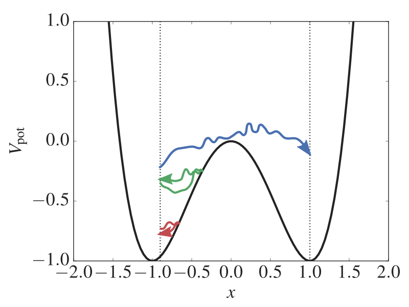
Fig. 27 The potential energy as a function of the position. We have two stable states (at x = -1 and x = 1) separated by a barrier (at x = 0). In addition, three paths are shown. One is reactive while the two others are not able to escape the state at x = -1. Using the RETIS method, we can generate such paths which gives information about the reaction rate and the mechanism. The vertical dotted lines show two RETIS interfaces.

Using the RETIS algorithm, we will set up the path ensembles, replica exchange moves, and analysis needed to estimate the rate constant for the transition between the two states. This particular problem has been considered before by van Erp [1] [2]; the focus here is how to adapt the setup for your own rare-event simulations.

Verification status: passing – see Tutorial map.

Tutorial quick start

• Best starting point: examples/tutorials/path_sampling/internal/1D-double-well/retis/.

• Edit first: retis.toml for interfaces, move settings, engine settings, and output frequency; edit initial.xyz only when changing the system.

• Run: pyretis run -i retis.toml -p.

• Analyse: pyretis analyse -i retis.toml – the analysis reads the same input file as the run.

• Expected output: numbered ensemble folders, trajectory/order/energy files, pyretis.log, output.toml, and a report/ folder after analysis.

• Related checks: examples/tests/test-internal/retis/, examples/tests/test-internal/retis-restart/, and examples/tests/test-internal/retis-load-sparse/; see Example test status.

Creating the PyRETIS input file

We will now create the input file for PyRETIS. We will do this section by section in order to explain the different keywords and settings. The full input file is given at the end of this section.

Setting up the simulation task

The first thing we will define is the type of simulation we will run. This is done by creating a simulation section.

Here, we are going to do a retis simulation and we will do 20000 steps [2]. Since we will be running a path sampling simulation, we will also need to specify the positions of the interfaces we will be using.

[simulation]
task = "retis"
steps = 20000
interfaces = [
    -0.9,
    -0.8,
    -0.7,
    -0.6,
    -0.5,
    -0.4,
    -0.3,
    1.0,
]

Setting up the system

We will now set up the system we are going to consider. Here, we will actually define several PyRETIS input sections:

• The system section which defines the units, dimensions and temperature we are considering:

  [system]
  units = "reduced"
  dimensions = 1
  temperature = 0.07
  

• The box section, but since we are here just considering a single particle in a 1D potential, we will simply use a 1D box without periodic boundaries:

  [box]
  periodic = [
      false,
  ]
  

• The particles section which add particles to the system and defines the initial state:

  [particles]
  name = [
      "Ar",
  ]
  ptype = [
      0,
  ]
  
  [particles.position]
  input_file = "initial.xyz"
  
  [particles.velocity]
  generate = "maxwell"
  momentum = false
  seed = 0
  
  [particles.mass]
  Ar = 1.0
  

  In this case, we will read the initial configuration from a file initial.xyz and velocities are generated from a Maxwell distribution. Further, we specify the mass, particle type and we label the particle as Ar. Note that this does not mean that we are simulating Argon, it is just a label used in the output of trajectories.

• The force field and potential sections which setup up the 1D double well potential:

  potential = [
      { class = "DoubleWell", a = 1.0, b = 2.0, c = 0.0 },
  ]
  [forcefield]
  description = "1D double well"
  

Selecting the engine

Here, we will make use of a stochastic Langevin engine. We set it up by setting the time step, the friction parameter and whether we are in the high friction limit. The seed given is a seed for the random number generator used by the integrator.

[engine]
class = "Langevin"
timestep = 0.002
gamma = 0.3
high_friction = false
seed = 0

TIS specific settings

The TIS settings control how the TIS algorithm is carried out. Here we set that 50 % of the TIS moves should be shooting moves (keyword freq) and we limit all paths to a maximum length of 20 000 steps. Further, sigma_v = -1 selects aimless shooting. We also tell PyRETIS to not set the momentum to zero and to not rescale the energy after drawing new random velocities. We also set allowmaxlength = False which means that for shooting, we determine stochastically the length of new paths based on the length of the path we are shooting from. The given seed is a seed for the random number generator used by the TIS algorithm.

[tis]
freq = 0.5
maxlength = 20000
allowmaxlength = false
zero_momentum = false
rescale_energy = false
sigma_v = -1
seed = 0

RETIS specific settings

The RETIS section controls the RETIS algorithm. Here swapfreq = 0.5 is the probability that a move picked in the \([0^-]\) or the \([0^+]\) ensemble is the swap of the paths of the two (the zero swap), when the other ensemble is free.

[retis]
swapfreq = 0.5

Initial path settings

These settings determine how we find the initial path(s). Here, we ask PyRETIS to generate these using the kick method.

[initial-path]
method = "kick"
kick-from = "initial"

Selecting the order parameter

For this system, we simply define the order parameter as the position of the single particle we are simulating.

[orderparameter]
class = "pyretis_position"
dim = "x"
index = 0
periodic = false

Modifying the output

In the Output section, we here keep the trajectory of only every 100th path the run replaces in the archive (archive_every). A value above 0 of energy-file and order-file writes the energies and the order parameter of each path.

[output]
archive_every = 100
energy-file = 100
order-file = 100

Show/hide the full input file »

potential = [
    { class = "DoubleWell", a = 1.0, b = 2.0, c = 0.0 },
]

[simulation]
task = "retis"
steps = 20000
interfaces = [
    -0.9,
    -0.8,
    -0.7,
    -0.6,
    -0.5,
    -0.4,
    -0.3,
    1.0,
]

[system]
units = "reduced"
dimensions = 1
temperature = 0.07

[engine]
class = "Langevin"
timestep = 0.002
gamma = 0.3
high_friction = false
seed = 0

[box]
periodic = [
    false,
]

[particles]
name = [
    "Ar",
]
ptype = [
    0,
]

[particles.position]
input_file = "initial.xyz"

[particles.velocity]
generate = "maxwell"
momentum = false
seed = 0

[particles.mass]
Ar = 1.0

[forcefield]
description = "1D double well"

[orderparameter]
class = "pyretis_position"
dim = "x"
index = 0
periodic = false

[output]
archive_every = 100
energy-file = 100
order-file = 100

[tis]
freq = 0.5
maxlength = 20000
allowmaxlength = false
zero_momentum = false
rescale_energy = false
sigma_v = -1
seed = 0

[initial-path]
method = "kick"
kick-from = "initial"

[retis]
swapfreq = 0.5

Running the RETIS simulation

We will now run the RETIS simulation. Create a new directory and place the input file (let’s call it retis.toml) here. Also, download the initial configuration initial.xyz and place it in the same folder. The simulation can then be executed using:

pyretis run -i retis.toml -p

The -p option will display a progress bar for your simulation.

Analysing the results

When the simulation has finished, we can analyse the results. The analysis reads the same input file as the run; the run itself writes output.toml, which records the input it ran with, under the names of the input and with every default included. pyretis analyse -i output.toml reads the input sections from it and gives the same analysis.

How the analysis is performed is controlled by an analysis section, which you can add to the input:

Analysis settings
-----------------
maxordermsd = -1
ngrid = 1001
report = ['latex', 'rst', 'html']
maxblock = 1000
txt-output = 'txt.gz'
blockskip = 1
plot = {'output': 'png', 'plotter': 'mpl', 'style': 'pyretis'}
bins = 100
skipcross = 1000

For a description of these keywords, we refer to the analysis section.

The analysis itself is performed using:

pyretis analyse -i retis.toml

This will produce a new folder, report which contains the results from the analysis. If you have latex installed, you can generate a pdf using the file retis_report.tex within the report folder. An example result for the crossing probability is shown below.

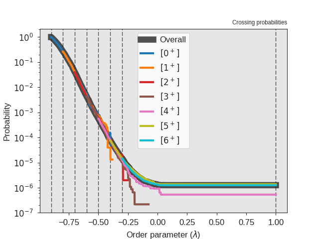
Fig. 28 Sample output from the analysis. This figure shows the crossing probabilities for the individual ensembles and the overall crossing probability.

Improving the statistics

We can improve the statistics by running a longer simulation. To continue the simulation in its directory up to 1000000 steps, set method = "restart" in the [initial-path] section and steps = 1000000 in the [simulation] section of retis.toml, run

pyretis run -i retis.toml -p

again, and repeat the analysis. The restart continues from the cycle and the paths saved in output.toml and appends the new cycles to the output of each ensemble (see the restart method). Running the input again with method = "kick" in the same directory stops with an error, since its ensemble directories hold the sampled cycles. To start over, use a new directory, or first run pyretis tools clean (see Cleaning run artifacts). Below we show an example for the crossing probability after performing the additional steps

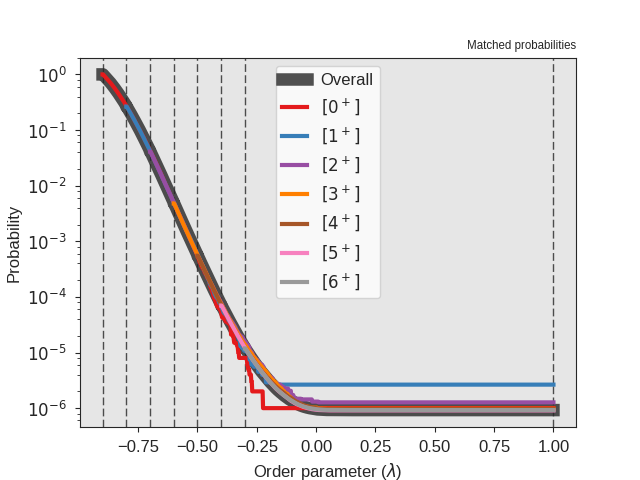
Fig. 29 Sample output from the analysis. This figure shows the crossing probabilities for the individual ensembles and the overall crossing probability after running 1000000 steps.

Tested by

The main workflow is represented by examples/tests/test-internal/retis/. Restart and loading behavior are covered by examples/tests/test-internal/retis-restart/ and examples/tests/test-internal/retis-load-sparse/. These checks are shorter than the tutorial run but exercise the same input parsing, simulation, and analysis path.

References

[1]

Titus S. van Erp, Dynamical Rare Event Simulation Techniques for Equilibrium and Nonequilibrium Systems, Advances in Chemical Physics, 151, pp. 27-60, 2012, https://doi.org/10.1002/9781118309513.ch2

[2] (1,2)

https://arxiv.org/abs/1101.0927