Post-processing and visualization with PyVisA

In this example, we perform post-processing on the methane hydrate system from one of the previous examples called “Using GROMACS”. All post-processing is done with the PyVisA analysis tab, shown in Fig. 51, and the recalculation tool. We will continue the study of cage-to-cage diffusion within a S1 hydrate and add new collective variables. Then we perform clustering, principal component analysis (PCA), and visualization of the new results. These analysis methods require the scikit-learn and scipy packages.

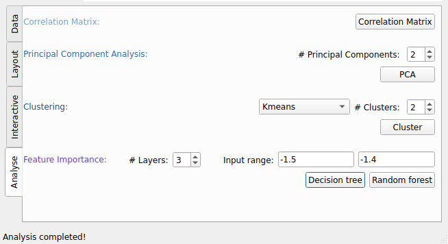
Fig. 51 Analysis tab of PyVisA with options for interactivity, animation, and post-processing.

Before we proceed with the analysis, we need to have some simulation results, so please run the example Using GROMACS first.

The example is structured as follows:

Visualization and compression

When the simulation has finished, the results can be visualized and post-processed. It is always important to save the original data, because the recalculation creates new PyVisA data from the trajectory files of the old simulation. This loses the frames between stored trajectory files. The following steps are suggested:

1. Compress the original data into an HDF5 file using:

   pyvisa -i out.rst -cmp
   

2. Compress only the order parameter data into an .hdf5.zip file using:

   pyvisa -i out.rst -cmp -oo
   

3. Rename these files to standard_simulation.hdf5.zip.

The results can be visualized from the .rst files or from the compressed files. If you want to visualize the data, the following commands can be run:

pyvisa -i <input-file>

pyvisa -i <rst-file> -data <data>

where <input-file> can be either an .rst file or an .hdf5.zip file. If you are using the -data command, then <data> can be all to load all data, a trajectory file, or a simulation directory. For example, the first path ensemble can be loaded by using 000 as <data>.

With PyVisA, you can visualize trajectories from all path ensembles and sort them by status and Monte Carlo move. Try finding and visualizing a reactive pathway by clicking on the plot and pressing “Show trj” in the Analysis tab. This highlights the points that belong to the selected trajectory. You can also customize how the visualization looks. In Fig. 52 a reactive pathway has been shown.

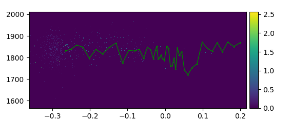
Fig. 52 Density plot of the order parameter and the kinetic energy from the methane hydrate example with a reactive pathway shown in green.

Recalculation of new collective variables

Now that the old data has been stored, we can add two more collective variables to the simulation using PyVisA. The collective variables we introduce are the area of the six-membered ring that the methane jumps through, and the volume of the starting cage. These descriptors will try to capture the breathing of the starting cage. The following lines must be added to the retis.rst file:

Collective-variable
-------------------
class = AreaAndVolume
module = orderp.py

With the collective variable added to retis.rst, we also need to add the Python script for the calculation in the orderp.py file. The scipy package is needed to run this script, so make sure that it is installed. The full script is given here:

Show/hide the Python script for the new collective variable. »

import logging
import numpy as np
from scipy.spatial import ConvexHull
from pyretis.orderparameter import OrderParameter
logger = logging.getLogger(__name__)  # pylint: disable=invalid-name
logger.addHandler(logging.NullHandler())


class AreaAndVolume(OrderParameter):
    """AreaAndVolume(OrderParameter).

    This order parameter calculates the area of the six-membered ring
    which the methane molecule jumps through when performing the L6L jump,
    and the volume of the starting cage.

    Attributes:
    ----------
    periodic : boolean
        This determines if periodic boundaries should be applied to
        the position or not.

    """

    def __init__(self, periodic=True):
        """Initialize the class."""
        super().__init__(description="Area of ring and volume "
                                     "of starting cage")
        self.periodic = periodic
        self.idx1 = np.array([220, 252, 412, 444, 796], dtype='i4')
        self.idx2 = np.array([220, 252, 284, 316, 412, 444, 540, 604,
                              668, 700, 796, 828, 924, 988, 1052, 1084,
                              1180, 1212, 1308, 1340, 1372, 1404, 1436, 1468],
                             dtype='i4')

    def calculate(self, system):
        """Calculate area and volume."""
        pos = system.particles.pos
        ar_ring = ConvexHull(pos[self.idx1]).area
        vol_cage = ConvexHull(pos[self.idx2]).volume
        return [ar_ring, vol_cage]

As we also have the z-coordinate of the methane molecule as a collective variable, we add this to orderp.py so that the recalculation tool can use it. The Position descriptor is shown here:

Show/hide the Python script for the Position collective variable. »

class Position(OrderParameter):
    """A positional order parameter.

    This class defines a very simple order parameter which is just
    the position of a given particle.

    Attributes
    ----------
    index : integer
        This is the index of the atom which will be used, i.e.
        ``system.particles.pos[index]`` will be used.
    dim : integer
        This is the dimension of the coordinate to use.
        0, 1 or 2 for 'x', 'y' or 'z'.
    periodic : boolean
        This determines if periodic boundaries should be applied to
        the position or not.

    """

    def __init__(self, index, dim='x', periodic=False):
        """Initialise the order parameter.

        Parameters
        ----------
        index : int
            This is the index of the atom we will use the position of.
        dim : string
            This select what dimension we should consider,
            it should equal 'x', 'y' or 'z'.
        periodic : boolean, optional
            This determines if periodic boundary conditions should be
            applied to the position.

        """
        txt = 'Position of particle {} (dim: {})'.format(index, dim)
        super().__init__(description=txt, velocity=False)
        self.periodic = periodic
        self.index = index
        self.dim = {'x': 0, 'y': 1, 'z': 2}.get(dim, None)
        if self.dim is None:
            msg = 'Unknown dimension {} requested'.format(dim)
            raise ValueError(msg)

    def calculate(self, system):
        """Calculate the position order parameter.

        Parameters
        ----------
        system : object like :py:class:`.System`
            The object containing the positions.

        Returns
        -------
        out : list of floats
            The position order parameter.

        """
        particles = system.particles
        pos = particles.pos[self.index]
        lamb = pos[self.dim]
        if self.periodic:
            lamb = system.box.pbc_coordinate_dim(lamb, self.dim)
        return [lamb]

To begin the recalculation, start PyVisA by loading all data with the modified retis.rst file:

pyvisa -i retis.rst

It is important to load PyVisA with the modified retis.rst file so the program knows what has been added. The recalculation can then be started from the PyVisA file menu by selecting “Recalculate data”. The warning shown in Fig. 53 will appear. Press yes if you have added the post-processing requirements to both retis.rst and orderp.py.

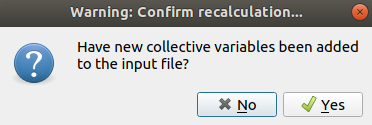
Fig. 53 The warning issued by PyVisA before the recalculations.

The recalculation will now start. When the procedure is finished, PyVisA loads the new data into the GUI and displays a message that the new data can be visualized.

Post-processing and clustering

Now that we have the new data, we can use PyVisA to perform clustering and PCA. The following steps can be done in the data exploration:

1. Go to the Analysis tab of PyVisA and press the button “Show correlations”. This will produce the correlation matrix. From these results, plot the order parameter and one of the collective variables.
2. Select a number of components to use in clustering and from the Analysis-selection, pick an algorithm for clustering and press the Analysis-button. This will produce a cluster plot of the chosen variables. Try to start with k-means, and then try Gaussian mixture and spectral clustering to see if there is a difference between the methods.
3. Try to perform a principal component analysis of the results. Begin by selecting 3 components, and PCA as the method, and press the analysis- button. This will produce the loading matrix, the scores plot from the first two components, and the cumulative explained variance. How much variance was retained? Were three components enough? Are there any strong correlations between the principal components and the original descriptors?

If you want to study the results from the principal component analysis further, the data will be stored in an HDF5 file in your simulation directory containing all the simulation data, and the data from the analysis.