Breaking a bond with RETIS and LAMMPS

In this example, you will explore bond breaking in a simple model system with the Replica Exchange Transition Interface Sampling (RETIS) algorithm. This example is similar to the Breaking a bond with RETIS example, but here, we will make use of LAMMPS for running the dynamics.

The system we consider consist of a simple diatomic bistable molecule immersed in a fluid of purely repulsive particles, as illustrated in Fig. 42.

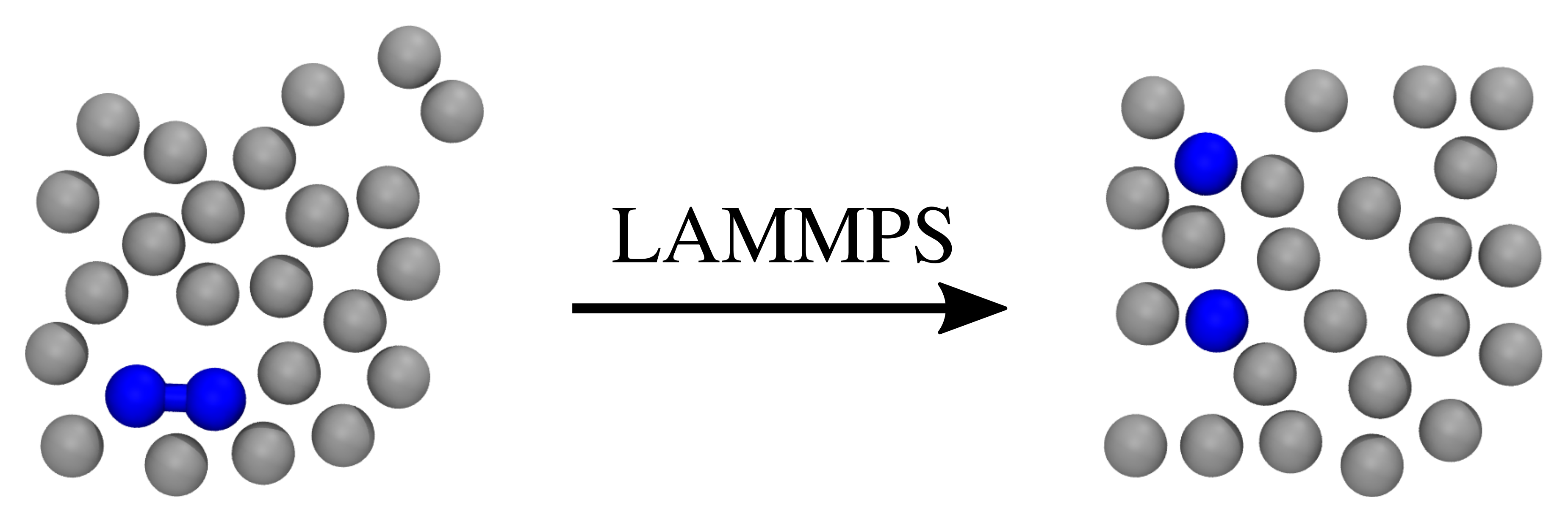
Fig. 42 Two snapshots of the system we consider here. The left snapshot illustrates a possible initial state, while the right snapshot illustrates a possible final state. Two of the particles (colored blue) are initially bound to each other, but this bond can break during the simulation. The gray particles represent the fluid in which the two bound particles are immersed in.

As mentioned in the Breaking a bond with RETIS example, this system was actually considered in the article introducing the TIS method, [1] and we will here largely follow this simulation set-up. We refer to the original article for more details. This example is structured as follows:

Defining the system, potential and order parameter

The system we will consider is a 2D system consisting of 25 particles at a fixed total energy of 1.0 per particle (in reduced units). The number density is set to 0.7. Between two of the particles, the “diatomic molecule”, we have a double well potential, given by

where , and . In addition, we have a Weeks-Chandler-Andersen (WCA) pair interaction between all particles. The potential functions are illustrated in Fig. 43. In this figure, we also show the interfaces we will consider for the RETIS method. These interfaces have been placed at the positions given in the original TIS article. [1]

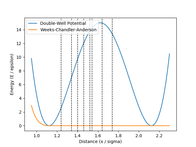
Fig. 43 The double well potential and the WCA pair interaction potential. The dashed lines show the interface positions we will consider for the RETIS method.

For the order parameter, we choose the distance between the two atoms which are initially bound. We will in the next section describe the input files needed to run this example with LAMMPS.

Preparing input files for LAMMPS

We will here follow the description given in the LAMMPS user guide. Thus we need to create:

• A LAMMPS input file for performing molecular dynamics: The LAMMPS input file to use with this example can be found here: lammps.in. We will not discuss this input script in detail, but we note the following:

  • We set two variables defining a temperature and energy (per particle): variable SET_TEMP equal 1.0 and variable SET_ENERGY equal 1.0. When performing the shooting move, we will draw velocities and scale them so that the total energy of the system is 1.0 per particle.
  • We include an external script, defining the double well potential: include "dw-wca.in" This file can be found here: dw-wca.in.

• A file containing initial coordinates: We load the initial coordinates from a file, system.data. This file can be found here: system.data. The box size is set to give a 2D particle density of 0.7 in reduced units.

• A LAMMPS input file for calculating the order parameter: The LAMMPS input file defining the order parameter is in this case rather simple:

  variable op_1 equal v_delr
  

  The file itself can be found here order.in. The file basically renames an already existing variable, delr, which is used in the potential energy calculation, to op_1, which is the variable name PyRETIS expects for the order parameter.

In total, we now have 4 files we will use to define the LAMMPS part of the PyRETIS simulation:

Table 53 LAMMPS input files needed for the example

File description	Filename/download
LAMMPS MD input file	lammps.in
Initial configuration	system.data
Order parameter definition	order.in
Definition of potential functions	dw-wca.in

Generating an initial trajectory

We need at least two initial trajectories for PyRETIS, which should satisfy some requirements for the order parameter as illustrated in Fig. 44.

The requirements for the initial trajectory in the ensemble are that:

1. The first and last points of the trajectory should be the only two points where the order parameter is larger than the value of the first interface.
2. The trajectory must be more than the first and last points.

These conditions imply that two interface crossing events occur during the trajectory, and that all points other than the first and last points have order parameter values less than the value of the first interface. An example satisfying these conditions is shown in green in Fig. 44.

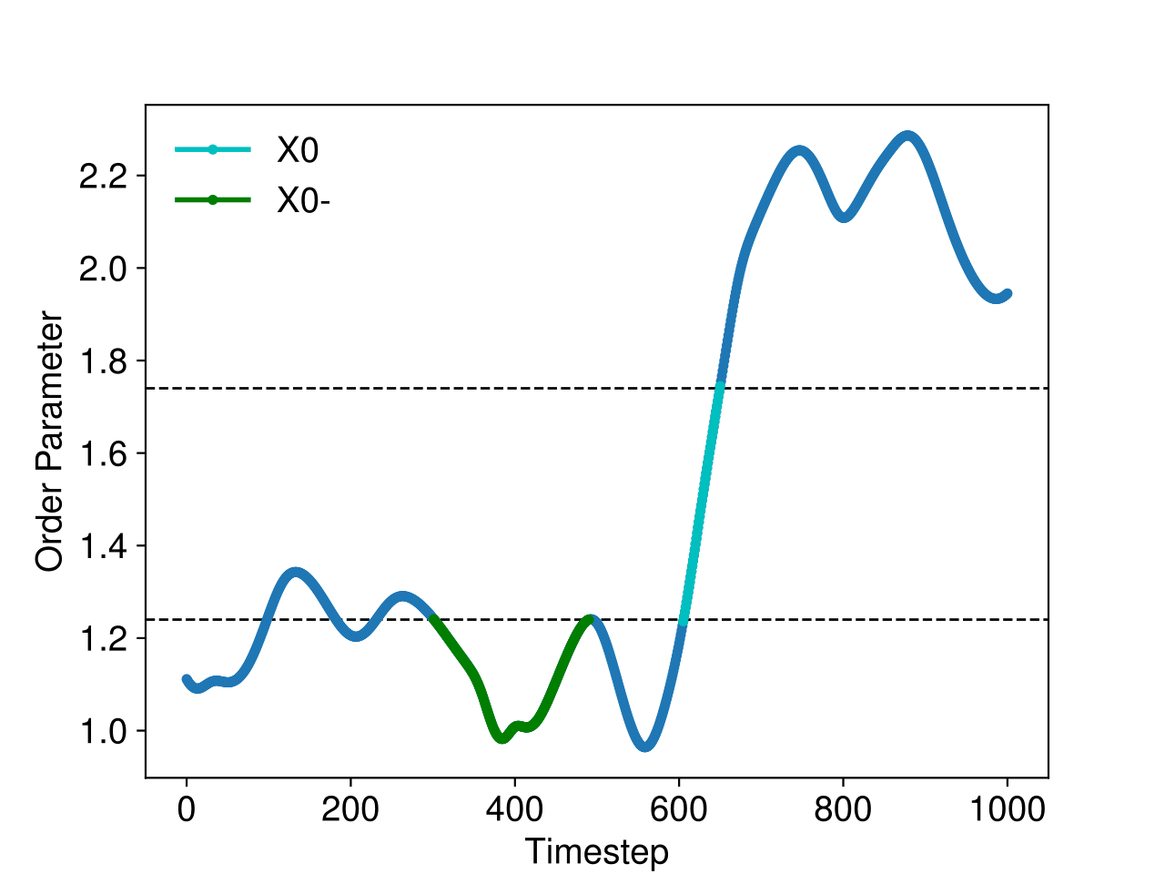
Fig. 44 The order parameter in a simulation containing a trajectory in the ensemble (green) and a crossing trajectory (cyan).

For an initial trajectory satisfying the requirements for all other ensembles, it is sufficient that:

1. The first point of the trajectory should have an order parameter value less than the value of the first interface.
2. The last point of the trajectory should have an order parameter value greater than the value of the last interface.
3. There must be at least one other point in addition to the first and last points in the trajectory, and these other points should all have order parameter values in between the values of the first and last interfaces.

These conditions imply that we would like to use a reactive trajectory as an initial trajectory. An example reactive trajectory is shown in cyan in Fig. 44.

Because the reactive condition is normally a rare event, we need to run a biased simulation in order to generate the initial reactive trajectory. In this case, because the reactive condition was distance based (distance between two atoms), we are able to use LAMMPS fix spring to pull the atoms apart:

fix pulling_simulation atom1 spring couple atom2 2.0 0.0 0.0 0.0 1.0

In this example, atom1 and atom2 are LAMMPS groups referring to the two atoms participating in the double well potential.

Running the RETIS simulation

After having generated an initial trajectory, we are ready to set up the simulation for PyRETIS. We will here use similar settings to the internal example for the same system, please see the Breaking a bond with RETIS example for a description of these settings. The full input script can be found here retis.rst. In the following, we will highlight the settings that are specific to using LAMMPS, and to loading the initial trajectory we have already generated.

Setting up the LAMMPS engine

The LAMMPS engine is defined with the following section,

Engine settings
---------------
class = lammps
lmp = lmp_serial
input_path = lammps_input
subcycles = 1
extra_files = ['dw-wca.in']

These lines assumes that we have stored the LAMMPS input files in a folder named lammps_input and that there is an “extra” file named dw-wca.in needed here. The term “extra” just refers to the fact that this file is in addition to the default files PyRETIS expects to find here. We also specify a specific name for the LAMMPS executable lmp = lmp_serial in this case. Note that this might have to be changed before running the example on your own computer.

Loading the initial path

Loading the previously obtained initial path can be done with the following section:

Initial-path
------------
method = load
load_folder = load

This assumes that the initial path is stored in a folder named load. In this folder, we create a sub-folder for each ensemble, load/000, load/001, …, load/007 and for each of these ensemble directories we include the files needed for the initial path. For a given ensemble this should include the following:

• A file named order.txt with the order parameters for the path.

• A file named traj.txt with information about the initial path: This includes information about the snapshots the initial path consist of. For each snapshot we need to specify the following:

  • the step number (“index”) in the path
  • the LAMMPS trajectory file that contains the snapshot
  • the index in the LAMMPS trajectory file that corresponds to the snapshot
  • a flag which tells PyRETIS if the velocities are to be reversed or not before PyRETIS can make use of it.

  The first few lines of such a file might look like:

  #     Step              Filename       index    vel
           0       cross.lammpstrj        1174     -1
           1       cross.lammpstrj        1175     -1
           2       cross.lammpstrj        1176     -1
           3       cross.lammpstrj        1177     -1
  

  Here, the first column lists the step number for the initial path, the second column contains information about what LAMMPS trajectory file to read, the third column tells PyRETIS what index in the given LAMMPS trajectory the snapshot corresponds to and the fourth (and final) column is the velocity flag. A -1 means that PyRETIS can use this snapshot without reversing the velocities, while a 1 means that PyRETIS will have to reverse velocities before using the snapshot.

• A directory named accepted which contains the LAMMPS trajectory file(s) the initial path is made up of.

Executing the RETIS simulation

Once all the input files have been assembled, the simulation can be executed using pyretisrun:

pyretisrun -i retis.rst -p

assuming that you named the main PyRETIS input file retis.rst.

Analyzing the RETIS results

After the simulation has finished, or while it is running, you can start analyzing the results. For instance, we can have a look at the accepted paths in the last (007) ensemble. These are stored in the folder 007/traj/traj-acc. In figure Fig. 45, we show the energies and the order parameter for such an accepted path:

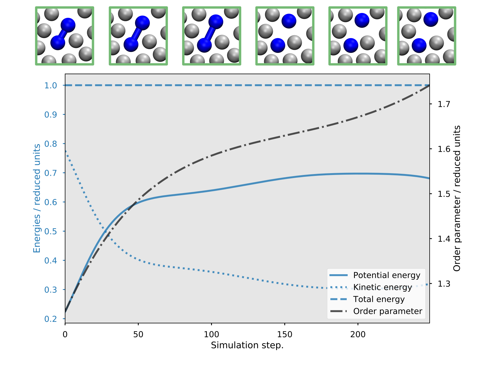
Fig. 45 Example of a reactive trajectory obtained by the RETIS simulations. This shows the energies and the order parameter as a function of the simulation step, along with a few selected snapshots.

Further, we can run an analysis to obtain the crossing probability and the rate of the transition. This can be done using the pyretisanalyse tool. While running the simulation a new file, out.rst, should have been created in the main directory. To use this file in the analysis, you will first have to insert the correct time step (i.e. the LAMMPS time step multiplied with the subcycles) into the Engine settings section of this file. As a specific example, for a LAMMPS time step of 0.001 and a subcycles setting of 1 in the original retis.rst input file, you should update the out.rst file to include the timestep setting. For instance:

Engine settings
---------------
timestep = 0.001

The analysis can then be executed using:

pyretisanalyse -i out.rst

This will produce several output files, which are summarized in a folder report in the main directory. Below you can find a table with some sample results and a figure showing the obtained crossing probability.

Table 54 Crossing probability, initial flux and the rate constate for an example run of the 2D WCA example with LAMMPS. The quantities are given in reduced units.

Quantity	Value	Relative error
Crossing probability	5.5e-12	24 %
Initial flux	0.1196	1 %
Rate constant	6.6e-13	24 %

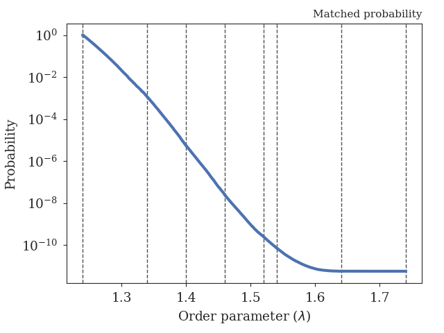
Fig. 46 The obtained crossing probability for the 2D WCA LAMMPS example. The dashed lines show the positions of the interfaces we have considered here.

References

[1]	(1, 2) Titus S. van Erp, Daniele Moroni, and Peter G. Bolhuis, A novel path sampling method for the calculation of rate constants, The Journal of Chemical Physics, 118, pp. 7762 - 7774, 2003.