Introduction to the PyRETIS library
In this introduction to the PyRETIS library the main classes and functions from the PyRETIS library will be discussed. For the full description, we refer to the API documentation.
The PyRETIS library contains methods and classes that handle the different aspects of a simulation. These are grouped into sub-packages and the different sub-packages and the classes and methods defined within them will interact. As an example, assume that we are performing a RETIS simulation. In terms of objects from the PyRETIS library, this simulation can be described as follows:
- We first define the
Systemwe are studying. This contains information about theParticles,Boxand theForceField. - Next, an
OrderParameteris defined and the order parameter it is representing can be calculated using aSystemobject as the argument. - The RETIS simulation is handled by the
SimulationRETISclass which will use a specificEngineBaselike object in order to generate severalPathobjects for a collection ofPathEnsembleobjects. This generation is done by a set of methods defined in the modulespyretis.core.tisandpyretis.core.retis. - An analysis is carried out by making use of methods from the
analysissub-package.
Table of Contents
The core and forcefield sub-packages
The pyretis.core library defines the core method and
classes and here we will introduce the
Systemclass which defines the system we are investigating. This class is actually composed of several other objects, which we will also discuss here:Particles: A class which represents the particles.Box: A class which represents the simulation box.ForceField: A class representing the force field. (Note: This is defined withinpyretis.forcefield).
Pathclass which defines paths/trajectories.PathEnsembleclass which defines path ensembles.
Below is an illustration of how some of these classes are interacting. The classes (shown as boxes in this figure) will be discussed more in the following.
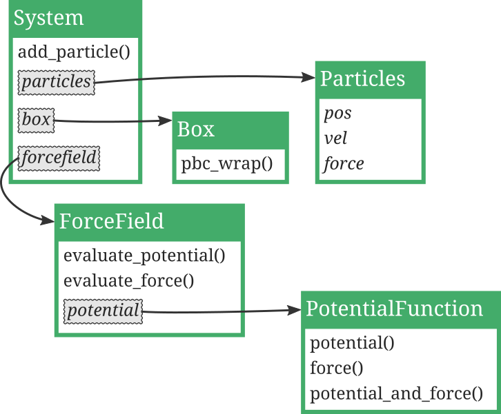
Fig. 10 Illustration of the relations between classes from the
core and force field sub-packages. The classes as shown as green
boxes where the class names are shown with white text.
Examples of class methods are written as “method()” while
and class attributes are indicated as just “attribute”. Some
of the attributes are in fact references to other classes and these are
highlighted with grey boxes and the reference is shown by arrows.
As can be seen in this figure, the System is in practice
composed of several other classes.
The System class
The System class
defines the system we are investigating. It will
typically contain particles, a simulation box and a
force field. This class exposes important parts we
can interact with, in particular, the particles.
Example of creation:
from pyretis.core import System
new_system = System(temperature=0.8, units='lj')
This will create an empty system with a set temperature equal to 0.8 in
lj units (lj refers to Lennard-Jones units).
It is also possible
to specify a box here in case that it needed:
new_system = System(temperature=0.8, units='lj', box=mybox)
where mybox can be created as
described below.
Particles can be added by first creating an object as described below. A short example:
from pyretis.core import System, Particles
new_system = System(temperature=0.8, units='lj')
new_system.particles = Particles()
new_system.add_particle([0.0, 0.0, 0.0], mass=1.0, name='Ar', ptype=0)
Here, we are setting the System.particles attribute and
using the System.add_particle() to add a particle with a given
position, mass, name and type.
The Particles class
The Particles class
represents a collection of particles and in many
ways it can be viewed as a particle list.
Internally in PyRETIS, the particle
list is one of the most important classes. The positions, velocities and
forces are accessed through an instance of this class using
the class attributes Particles.pos, Particles.vel and
Particles.force. Actually, there is an additional particle class
within PyRETIS which is called ParticlesExt. This class is
used when PyRETIS is using external engines. It is very similar to the
Particles class but it has, in addition, a
ParticlesExt.config which can be used to reference files
which hold the current configuration of the particles.
Here are some examples of interacting with
the Particles class,
using Particles.add_particle() to add
some particles. Actually, the system will make use of this
method if you are calling System.add_particle().
from pyretis.core import Particles

part = Particles(dim=3)

pos = [0.0, 1.0, 0.0]
vel = [0.0, 0.0, 0.0]
force = [0.0, 0.0, 0.0]
part.add_particle(pos, vel, force, mass=1.0, name='Ar', ptype=0)
print(part.pos)
pos = [1.0, 0.0, 0.0]
part.add_particle(pos, vel, force, mass=1.0, name='Ar', ptype=0)
print(part.pos)
Here, we can add names to particles using the keyword name and we
can also specify a particle type using ptype.
The name can be used to identify/tag
specific particles and is used for output purposes.
Internally, the particle type is more important:
The particle type can
be used to specify parameters for pair interactions which is computed
by the force field.
When we initiate an instance of Particles, we define the dimensionality
using the dim keyword parameter.
The Box class
The Box class
defines a simulation box. It is useful in
simulations where we wish to have periodic boundaries. Typically,
we do not interact much with the box beyond creating it.
Boxes are created by passing an (optional) cell argument which is a list
of floats of form [lengthx, lengthy, lengthz]. If more than
three floats are given, we assume that these represent a flattened version
of the box matrix of the form: [xx, yy, zz, xy, xz, yx, yz, xz, zy].
At the same time, periodicity can
be specified with the keyword periodic which is a list of boolean values
that determine if a dimension is periodic or not. The default is periodic
in all directions.
Some examples:
from pyretis.core import create_box
box1 = create_box()
print(box1)
box2 = create_box(cell=[10, 10, 10])
print(box2)
box3 = create_box(low=[0, -10, 10], high=[10, 10, 20],
                  periodic=[True, True, False])
print(box3)
The ForceField class
The ForceField class
is used to define force fields.
A force field is just a list of functions (and parameters)
which can be used to obtain the force and potential energy.
In general, the force field expect that its constituent potential functions
actually supports calling three functions which means that the
potential functions must be slightly more complex than just simple
functions — they need to be classes which
subclass the
PotentialFunction class.
If we, for the sake of an example,
let an instance of the ForceField class have a constituent potential
function named func, then PyRETIS will assume that it can call:
func.potential(system)to obtain the potential energy.func.force(system)to obtain the forces and the virial.func.potential_and_force(system)to obtain the potential energy, forces and the virial. Typically, this can be done by just callingfunc.potential(system)andfunc.force(system).
Notice that all these functions should only take in a System as
the only parameter.
Let’s see an example of how we can set-up a potential function (or class) and add it to a force field.
First, define the potential function using:
from matplotlib import pyplot as plt
import numpy as np
from pyretis.core import System, Particles
from pyretis.forcefield import ForceField
from pyretis.forcefield.potential import PotentialFunction


class Harmonic1D(PotentialFunction):
    """A 1D harmonic potential function."""

    def __init__(self):
        """Set up the potential."""
        super().__init__(dim=1, desc='1D harmonic potential')
        self.eq_pos = 0.0  # equilibrium position
        self.k_force = 1.0  # force constant

    def potential(self, system):
        """Calculate potential energy."""
        pos = system.particles.pos  # Get positions from the particle list.
        vpot = 0.5 * self.k_force * (pos - self.eq_pos)**2
        return vpot.sum()

    def force(self, system):
        """Calculate the force."""
        pos = system.particles.pos  # Get positions from the particle list.
        virial = None  # We are lazy and do not calculate the virial here.
        forces = -self.k_force * (pos - self.eq_pos)
        return forces, virial

    def potential_and_force(self, system):
        """Calculate force and potential."""
        pot = self.potential(system)
        force, virial = self.force(system)
        return pot, force, virial
Using what we have already discussed above about the System and Particles we can make a plot of the potential by adding:
if __name__ == '__main__':
    # Create empty force field:
    forcefield = ForceField(desc='1D Harmonic potential')
    pot = Harmonic1D()  # create potential
    # Add the potential function to the force field:
    forcefield.add_potential(pot)
    system = System()
    system.particles = Particles(dim=1)
    system.add_particle(pos=np.zeros(1))
    # Do some plotting, first calculate the potential as some locations:
    vpotentials = []
    positions = np.linspace(-2.5, 2.5, 100)
    for xi in positions:
        system.particles.pos = xi
        vpotentials.append(forcefield.evaluate_potential(system))
    # And plot it using matplotlib:
    fig = plt.figure()
    ax1 = fig.add_subplot(111)
    ax1.plot(positions, vpotentials, lw=3)
    plt.show()
The Path and PathEnsemble classes
These two classes are representations of paths and path ensembles.
Paths are essentially trajectories and path ensembles are collections of such
paths. The PathEnsemble stores some information about
all paths in the attribute PathEnsemble.paths, but
it will not store the full trajectory (positions, velocities, etc.).
It will, however, keep a reference to the last accepted path in
PathEnsemble.last_path. This Path object can,
for instance, be inspected by using the Path.phasepoints
attribute which is a list of system snapshots.
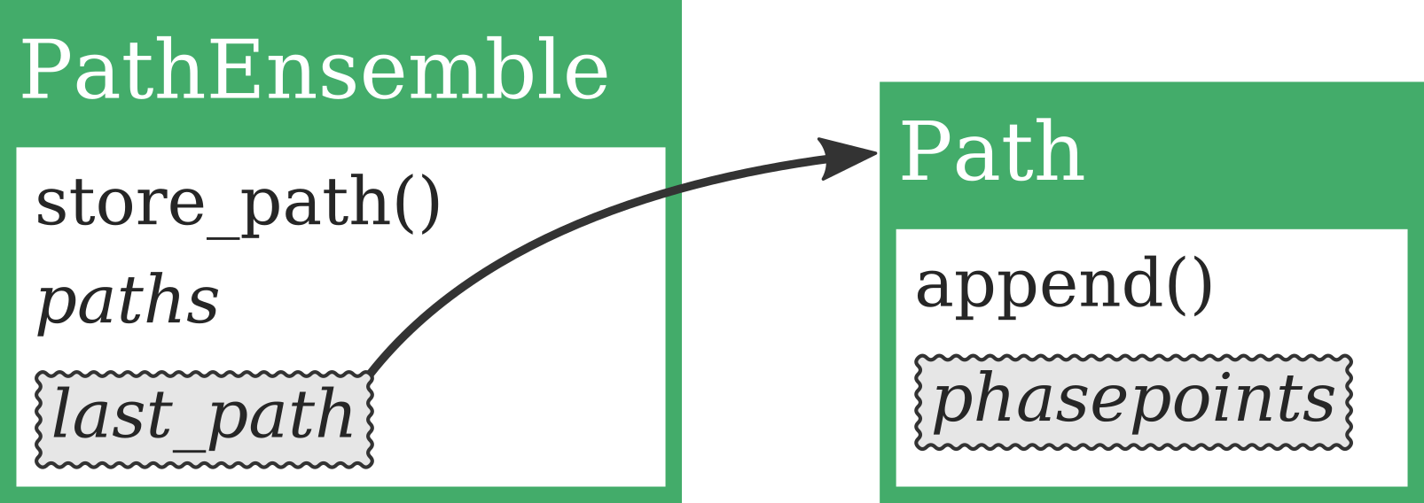
Fig. 11 Illustration of the relation between the
PathEnsemble and the Path.
We give here a short example on how you can interact with a path.
A complicating factor here is that we need to create a random
generator to use with the Path. This is done by using
the RandomGenerator class and the reader is referred to
the API documentation for information about this.
import numpy as np
from pyretis.core.system import System
from pyretis.core.particles import Particles
from pyretis.core.path import Path
from pyretis.core.random_gen import RandomGenerator

path = Path(rgen=RandomGenerator(seed=0))  # Create empty path.

# Add some phase points to the path:
for i in range(10):
    phasepoint = System()
    phasepoint.order = [i]
    phasepoint.particles = Particles(dim=3)
    phasepoint.add_particle(np.zeros(3), vel=np.zeros(3))
    phasepoint.vpot = i
    phasepoint.ekin = i
    path.append(phasepoint)

# Loop over the phase points in the path:
print('Looping forward:')
for i, phasepoint in enumerate(path.phasepoints):
    print('Point {}. Order parameter = {}'.format(i, phasepoint.order))

# Loop over the phase points in the path:
print('Looping backward:')
for phasepoint in reversed(path.phasepoints):
    print('Order parameter = {}'.format(phasepoint.order))

# Get some randomly chosen shooting points:
print('Generating shooting points:')
for i in range(10):
    point, idx = path.get_shooting_point()
    print(
        'Shooting point {}: index = {}, order = {}'.format(i, idx, point.order)
The simulation and engines sub-packages
The pyretis.simulation sub-package
defines classes which are used to set-up and define different types
of simulations. Typically, such simulations will need to interact
with and change the state of a given System. This
interaction is carried out by a particular engine object which behaves
like EngineBase
from the pyretis.engines sub-package.
The interaction between these classes are illustrated in the
figure below:
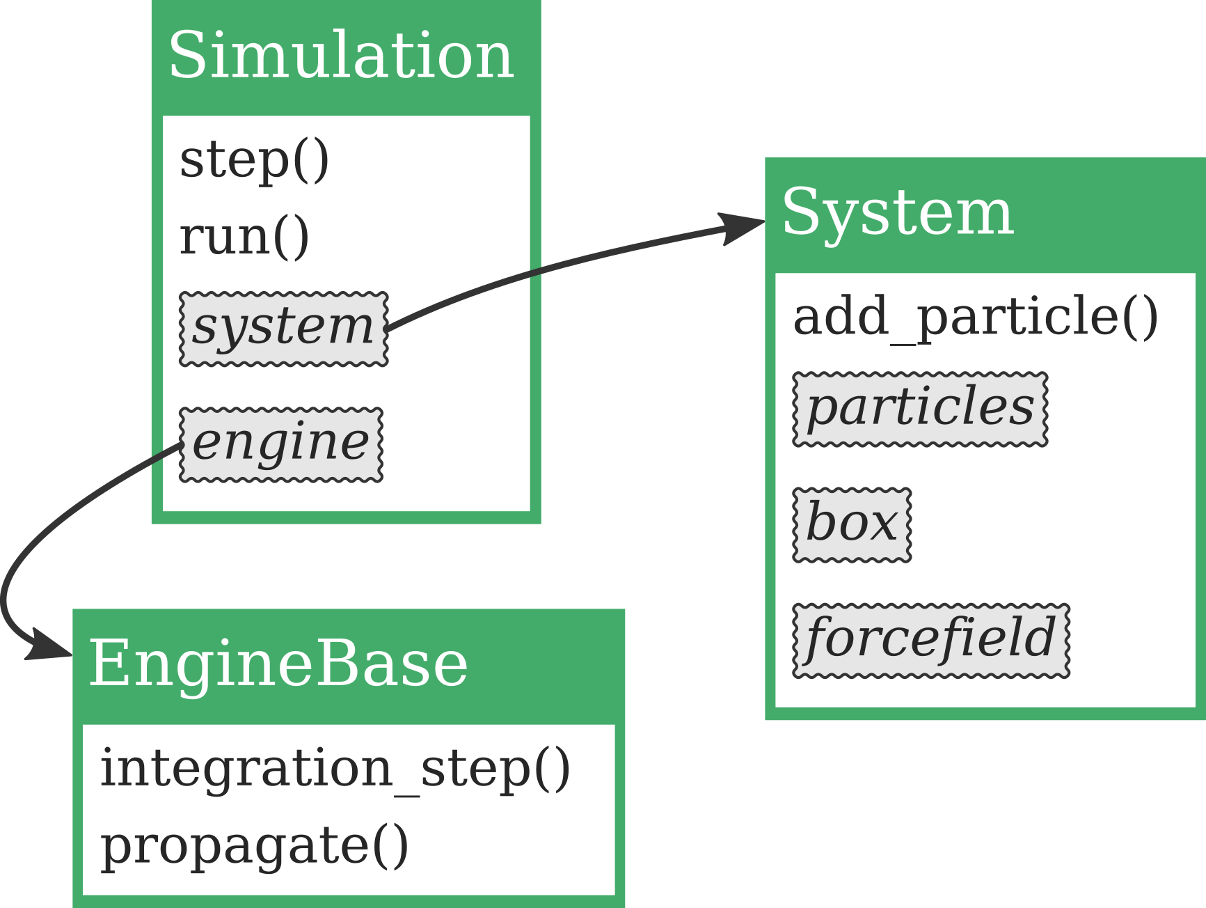
Fig. 12 Illustration of the relations between the Simulation,
EngineBase and System. A simulation object will
typically contain references to a system object and to an engine object. The
simulation can then use the engine in order to interact with the system. For
instance can the Simulation.step() methods use the
EngineBase.integration_step() in order to update positions, velocities
and forces in the system.
In this section, we will not give a complete example on how to create a new simulation class or a new engine class. We refer the reader to the examples, in particular:
- The section of the user guide which describes how new external engines can be interfaced.
- The particle swarm optimization example in
which a custom potential and engine is created. Further, in this example
a customized simulation is set up by making use of
Simulation.add_task() - The example showing how C for FORTRAN can be used to create a custom Velocity Verlet engine.
The Simulation class
The Simulation class defines a simulation we can run.
A simulation will typically act on a System
and alter its state. We will here just describe the generic
base class Simulation and we refer the reader to
the extended pyretis API documentation for
information about specific simulation classes, for instance,
the SimulationRETIS class. The most commonly
used methods from the Simulation are:
run()which will run a simulation and for each step it will yield a dictionary with results.step()which will run a single step from the simulation and return a dictionary with results.is_finished()which will returnTrueif the simulation has ended.add_task()which can be used to add simulation tasks to a generic simulation.
Example of creation:
from pyretis.simulation import Simulation
new_simulation = Simulation(startcycle=0, endcycle=100)

for step in new_simulation.run():
    print(step['cycle']['stepno'])
The code block above will create a generic simulation object and run it.
This simulation is not doing anything useful, it will only increment the
current simulation step number from the given startcycle to the
given endcycle. In order to something more productive, we can attach
tasks to the simulation. This can be done as follows:
from pyretis.core import System
from pyretis.simulation import Simulation


def function(sys):
    """Return the set temperature for the system."""
    return sys.temperature


simulation = Simulation(settings={}, controls={'steps': 10})
system = System(temperature=300)

my_task = {'func': function,
           'args': [system],
           'first': True,
           'result': 'temperature'}

simulation.add_task(my_task)

for result in simulation.run():
    step = result['cycle']['step']
    temp = result['temperature']['set']
    print(step, temp)
As you can see, a new task is added by defining it as a dictionary:
my_task = {'func': function,
           'args': [system],
           'first': True,
           'result': 'temperature'}
The following keywords are used:
funcwhich is a reference to a function to use.argswhich is a list of arguments that should be given to the function.firstwhether the task should be executed on the first simulation step (i.e. step 0).resulta string which labels the result in the dictionary returned by the methodsSimulation.run()orSimulation.step().
Typically, when creating a custom simulation, you will rewrite the
methods Simulation.run() and Simulation.step() to
fit the custom simulation you are going to perform, rather than adding
tasks. However, for interactive work, short examples etc.,
the Simulation.add_task() can be useful.
The EngineBase class
The EngineBase is a base class defining a generic
engine. In PyRETIS engines are either internal or external. External
engines, e.g. ExternalMDEngine,
interfaces external programs while
internal engines, e.g. MDEngine interact
directly with a System object. Creating an external engine
may be somewhat involved depending on the program you wish to interface.
A description on how to create new external engines can be
found in the user guide.
The orderparameter sub-package
The pyretis.orderparameter package defines order parameters
to use for path sampling simulation. In PyRETIS, such order parameters
are assumed to be functions of a System only. Here,
we give some examples of how a generic order parameter can be
used. For information on how custom order parameters can be
created, we refer to the detailed description in
the user guide.
The OrderParameter class
The most important piece of the OrderParameter class
is the actual calculation of the order parameter. This should be
defined in a method like OrderParameter.calculate().
Here, it is assumed that the order parameter takes in an object
like System. Since this is described
elsewhere we will here just describe
the usage of:
OrderParameter.calculate()which is used to calculate the order parameters.CompositeOrderParameterwhich can be used to combine several collective variables (e.g. when you are interested in additional order parameters).
First, we create an order parameter. For simplicity we use the pre-defined
Position class:
from pyretis.core import System, Particles
from pyretis.orderparameter import Position

position = Position(0, dim='x')
Next, we can calculate the order parameter as follows (the system we set up here is just for testing):
# Define a simple system for testing:
system = System()
system.particles = Particles(dim=3)
system.add_particle([1.0, 2.0, 3.0], mass=1.0, name='Ar', ptype=0)
print('Order =', position.calculate(system))
Several order parameters can be combined by creating
a CompositeOrderParameter. Below is an
example of how this can be used:
# -*- coding: utf-8 -*-
# Copyright (c) 2023, PyRETIS Development Team.
# Distributed under the LGPLv2.1+ License. See LICENSE for more info.
"""Example of interaction with a Composite order parameter."""
import numpy as np
from pyretis.core import System, Particles
from pyretis.orderparameter import (
    OrderParameter,
    Position,
    CompositeOrderParameter,
)

# Create a new, empty, order parameter:
order_parameter = CompositeOrderParameter()

# Add a position order parameter:
order_parameter.add_orderparameter(Position(0, dim='x'))

# Add a custom order parameter:
position_y = OrderParameter(description='Position along y-axis')


def collective_y(system):
    """Position along y-axis."""
    return [system.particles.pos[0][1]]


position_y.calculate = collective_y
order_parameter.add_orderparameter(position_y)

# Add another order parameter:
position_cos = OrderParameter(description='Cosine of z-coordinate')


def collective_cos(system):
    """Additional collective variable."""
    return [np.cos(np.pi * system.particles.pos[0][2])]


position_cos.calculate = collective_cos
order_parameter.add_orderparameter(position_cos)

# Create a system for testing the new order parameter:
i_sys = System()
i_sys.particles = Particles(dim=3)
i_sys.add_particle([1.0, 2.0, 3.0], mass=1.0, name='Ar', ptype=0)
print('Order =', order_parameter.calculate(i_sys))
Important
The first order parameter returned from
calculate() is taken as the
progress coordinate used in path sampling simulations.
The analysis sub-package
The pyretis.analysis sub-package defines tools which
are used in the analysis of simulation output. It defines methods
for running predefined analysis tasks, e.g. retis_flux(), but
also generic analysis methods, e.g. running_average().
Here, we refer the reader to the
pyretis API documentation for more
information about these methods.
The inout sub-package
The pyretis.inout sub-package contains methods which
PyRETIS make use of in order to interact with you.
These are ways to read input from you and to present output to you.
This sub-package is relatively large and it is in fact made up by
the following sub-packages:
pyretis.inout.analysisiowhich handles the input and output needed for analysis.pyretis.inout.formatsfor formatting and presenting text-based output.pyretis.inout.plottingwhich handles plotting of figures. It defines simple things like colors etc. for plotting. It also defines functions which can be used for specific plotting by the analysis and report tools.pyretis.inout.reportwhich is used to generate reports with results from different simulations.
Again, we refer to the pyretis API documentation for more information about these sub-packages.
The initiation sub-package
The pyretis.initiation sub-package contains methods to
initialize path ensembles. We refer the reader to the
pyretis API documentation for more
information about this sub-package.
The setup sub-package
The setup library contains methods to construct the main objects of PyRETIS from settings and from restart info.
The pyretis.setup which handles creation of objects
from simulation settings.
pyretis API documentation for more
information about this sub-package.
The tools sub-package
The tools library can be used to generate initial structures for a
simulation. In the tools library the function generate_lattice()
is defined and it supports the creation of the following lattices where
the shorthand keywords (sc, sq etc.) are used to select a
specific lattice:
sc: A simple cubic lattice.sq: Square lattice (2D) with one atom in the unit cell.sq2: Square lattice with two atoms in the unit cell.bcc: Body-centered cubic lattice.fcc: Face-centered cubic lattice.hcp: Hexagonal close-packed lattice.diamond: Diamond structure.
A lattice is generated in the following way:
from pyretis.tools import generate_lattice
xyz, size = generate_lattice('diamond', [1, 1, 1], lcon=3.57)
Where the first parameter selects the lattice type, the second parameter
selects give the number of repetitions in each direction and the optional
parameter lcon is the lattice constant. The returned values are
xyz – the coordinates – and size which is the bounding box of the
generated structure. This variable can be used to define a simulation box.
It is also possible to specify a number density:
from pyretis.tools import generate_lattice
xyz, size = generate_lattice('diamond', [1, 1, 1], density=1)
If the density is specified, the lattice constant lcon is deduced:
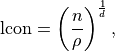
where  is the number of particles in the unit cell,
 the specified number density and
  the dimensionality.
If we wish to save a generated lattice, this can be done as follows
the dimensionality.
If we wish to save a generated lattice, this can be done as follows
from pyretis.tools import generate_lattice
from pyretis.inout.formats.xyz import write_xyz_file
xyz, size = generate_lattice('diamond', [3, 3, 3], lcon=3.57)
write_xyz_file('diamond.xyz', xyz, names=['C']*len(xyz), header='Diamond')

xyz, size = generate_lattice('hcp', [3, 3, 3], lcon=2.5)
name = ['A', 'B'] * (len(xyz) // 2)
write_xyz_file('hcp.xyz', xyz, names=name, header='HCP test')

xyz, size = generate_lattice('sq2', [3, 3], lcon=1.0)
write_xyz_file('sq2.xyz', xyz, header='sq2 test')
Some examples of using the PyRETIS library
Here, we show some examples of how we can perform some common tasks using the PyRETIS library.
Reversing a trajectory
PyRETIS will not reverse backward trajectories during a simulation if you are using an external engine. For visualization purposes, it is very helpful to reverse these trajectories before viewing them. This can be accomplished with the PyRETIS library as follows:
For GROMACS .trr trajectories:
from pyretis.inout.formats.gromacs import reverse_trr
reverse_trr('trajB.trr', 'rev-trajB.trr')
which will read the trajectory
trajB.trrand store it asrev-trajB.trr.For .xyz trajectories:
from pyretis.inout.formats.xyz import reverse_xyz_file
reverse_xyz_file('trajB.xyz', 'rev-trajB.xyz')
which will read the trajectory
trajB.xyzand store it asrev-trajB.xyz.
Recalculating order parameters
If you have an existing trajectory and with to calculate order parameters
for each step in the trajectory, this can be accomplished by making use of
the pyretis.tools.recalculate_order
module. For example, if you have a trajectory named traj.trr and
an order parameter defined in an input file retis.rst this can be
done as follows:
from pyretis.inout.formats.order import OrderFile
from pyretis.inout.settings import parse_settings_file
from pyretis.inout.setup import create_orderparameter
from pyretis.tools.recalculate_order import recalculate_order

settings = parse_settings_file('retis.rst')
order_parameter = create_orderparameter(settings)
options = {'reverse': False, 'maxidx': None, 'minidx': None}
order = recalculate_order(order_parameter, 'traj.trr', options)

with OrderFile('order.txt', 'w') as outfile:
    outfile.write('# Order parameters')
    for step, data in enumerate(order):
        print(step, data)
        outfile.output(step, data)
This will create a new file order.txt with the re-calculated order parameters.
The keyword reverse can be used to tell PyRETIS that you are looking at a
time-reversed trajectory. The keyword minidx gives the frame number from
which we start calculating (None is equal to reading from the first frame)
and the keyword maxidx gives the last frame number we will read (setting
it to None will read until the end of the trajectory file).