Introduction to PyRETIS and rare event methods
PyRETIS is a computational library for performing molecular simulations of rare events with a focus on transition interface sampling (TIS) [1] and replica exchange transition interface sampling (RETIS) [2].
Rare events are called rare because they happen at time or length scales much longer than we are able to simulate through brute-force simulations. Raindrops form every day, but compared to the motion of water molecules, raindrop formation is rare, and simulating it through brute-force simulations would take forever and a day.
Rare event methods aim to sample these rare events inaccessible through brute-force simulation.
Transition Interface Sampling
To explain the basic concepts, we consider an illustrative example: The transition between two stable states, from the reactant (labeled A) to the product (labeled B) as illustrated in Fig. 1.
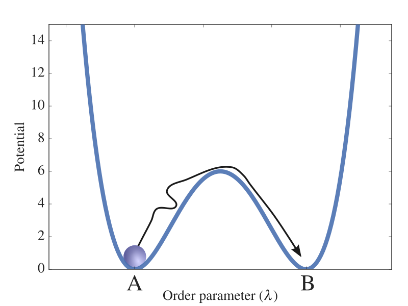
Fig. 1 A potential energy barrier separating two stable states A and B. The order parameter measures the extent of the reaction in this particular energy landscape and a possible trajectory for a particle making the transition is illustrated as a black arrow.
These two states are defined by a progress
coordinate (or order parameter),  ,
where state A is for
,
where state A is for  and state B for
  .
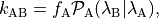
The central quantity calculated in TIS/RETIS simulations is the
rate constant
.
The central quantity calculated in TIS/RETIS simulations is the
rate constant  for the transition
 which can be expressed as:
and we see that it contains two parts:
- The initial flux
 which measures how often
trajectories start off at the foot of the reaction barrier
from the reaction side
which measures how often
trajectories start off at the foot of the reaction barrier
from the reaction side  . In TIS this
is obtained from a molecular dynamics (MD) simulation which
in PyRETIS is requested by running a
md-flux simulation. Note
that this is not needed for the RETIS method as explained.
. In TIS this
is obtained from a molecular dynamics (MD) simulation which
in PyRETIS is requested by running a
md-flux simulation. Note
that this is not needed for the RETIS method as explained. - The crossing probability
 of reaching
  before
given that has just been crossed.
In PyRETIS this can be accomplished by running a
tis or
retis simulation.
before
given that has just been crossed.
In PyRETIS this can be accomplished by running a
tis or
retis simulation.
As this is a rare event, the crossing probability is
extremely small and nearly impossible to compute in brute-force simulations.
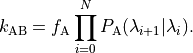
Transition interface sampling divides the region between A and B into
sub-regions using interfaces, denoted  (see Fig. 2).
The first interface,
(see Fig. 2).
The first interface,  is positioned at the interface defining
state A (
is positioned at the interface defining
state A ( ), and
the next interface,
), and
the next interface,  is put
at
is put
at  such that the probability of reaching
from is no longer extremely small. We can
continue in this fashion and place
such that the probability of reaching
from is no longer extremely small. We can
continue in this fashion and place  more interfaces until we
reach
more interfaces until we
reach  . What we effectively have
done with these
. What we effectively have
done with these  interfaces is to split up the
computation of the extremely small crossing probability into the
computation of many, not-so small, crossing probabilities:
interfaces is to split up the
computation of the extremely small crossing probability into the
computation of many, not-so small, crossing probabilities:
Here, the intermediate crossing probabilities,
 ,
are formally defined as the
probability of a path crossing
,
are formally defined as the
probability of a path crossing
 given
that it originated from ,
ended in or , and had
at least one crossing with in the past.
given
that it originated from ,
ended in or , and had
at least one crossing with in the past.
The interfaces we have placed defines the so-called path ensembles.
A path ensemble comprises all possible
trajectories that start at the foot of reaction
barrier from the reactant side (),
end in it or at the product region () and
having reached a certain threshold value () between the start point
and the final point. This path ensemble is labelled as ![\left[i^{+} \right]](../_images/math/cfbb46901bcfb4251ad06932f46e60074e907bb2.png) .
The probabilities,
.
The probabilities,
 can then
be obtained as the fraction of paths in the
can then
be obtained as the fraction of paths in the ![\left[i^+\right]](../_images/math/fa9378cdebead48813d241688fba009fb92a3ae5.png) ensemble
that also cross .
ensemble
that also cross .
Fig. 2 Illustration of TIS interfaces placed along the order parameter
in a system where a potential energy barrier separates two stable
states A and B. The interfaces define different ensembles and here,
two trajectories are shown. One (black) is reactive, reaching the final state,
while the other (orange) just reaches the intermediate  interface.
What is left now, is to have an efficient way of generating trajectories for the various path ensembles. This is in fact done by making use of a selection of Monte Carlo (MC) moves. For TIS [1] we choose between two moves:
The shooting move which is adapted from the transition path sampling (TPS) shooting algorithm [3] [4] to allow variable trajectory length. In this move, we generate a new trajectory from an existing trajectory one by:
- Picking randomly one of the discrete MD steps in the present trajectory.
- Modifying the velocities of this phase point (e.g. by randomly drawing new velocities from a Maxwellian distribution).
- Generating a new trajectory from this new phase point by integrating (i.e. running MD simulations) forward and backward in time until A or B is reached. The new trajectory is then obtained by merging the backward and forward trajectories.
The new trajectory is accepted as part of
![[i^+]](../_images/math/926a713ad232a99d786c85433990260ac088e0b2.png) only if all the following criteria are satisfied:
only if all the following criteria are satisfied:- A detailed balance condition for the energy and path length. [1]
- It starts at
- It has at least one crossing with before ending in A or B.
The shooting move gives a much higher chance to generate a valid trajectory at each trial compared to simply starting from a random phase point within the reactant well.
The time reversal move which generates trajectories by simply changing the time direction of a path. [1]
These two moves are illustrated in Fig. 4.
Replica Exchange Transition Interface Sampling
The RETIS method is similar to TIS and employs both the shooting
and time reversal moves.
In addition, RETIS makes use of the swapping move and defines a
new ensemble ![[0^-]](../_images/math/cc3aed0ac8713c58b57956a2b488b12008889b7f.png) which consist of trajectories that explore the reactant state
(see the illustration in Fig. 3).
which consist of trajectories that explore the reactant state
(see the illustration in Fig. 3).
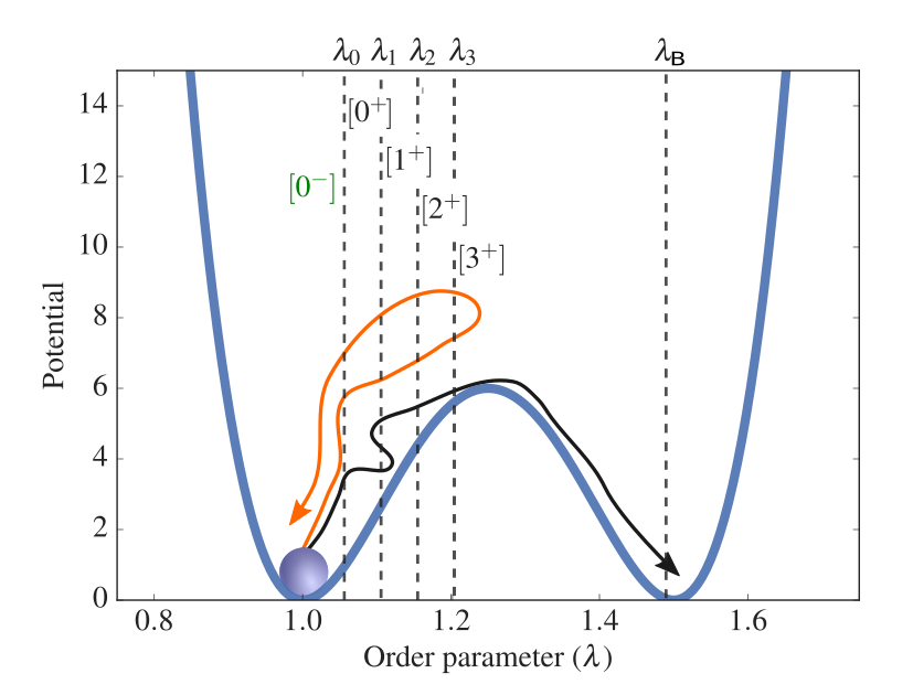
Fig. 3 Illustration of RETIS interfaces placed along the order parameter
in a system where a potential energy barrier separates two stable
states A and B. The interfaces define different ensembles and here,
two trajectories are shown. One (black) is reactive, reaching the final state,
while the other (orange) just reaches the intermediate
interface. In RETIS a special path ensemble, is also considered
as described in the text.
The swapping move acts between different path simulations. If two simulations generate simultaneously two paths that are valid for each other’s path ensemble, these two paths can be swapped. The swapping moves increase with negligible extra computational cost the number of accepted paths in the ensembles and decrease significantly the correlations between the consecutive paths within the same ensemble. All the moves used for generating trajectories are illustrated in Fig. 4.
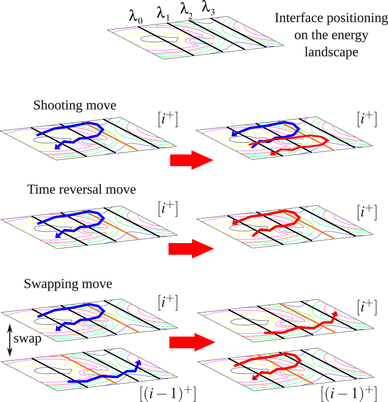
Fig. 4 Illustration of the RETIS moves for generating trajectories.
A contour plot of a hypothetical free energy
surface along a progress coordinate and an arbitrary second coordinate
is shown and 4 interfaces (, ,
and  ) have been positioned along the progress coordinate.
Three different RETIS moves (shooting, time reversal and swapping) are shown for
the
) have been positioned along the progress coordinate.
Three different RETIS moves (shooting, time reversal and swapping) are shown for
the ![[i^+] = [2^+]](../_images/math/8a5c164af564d57c1d05e529ffbe6b7061f1f8a6.png) path ensemble. The old paths are in blue and the new paths
after (a successful) completion of the MC moves are shown in red. The orange line
show the interface that needs to be crossed for a valid path in the current ensemble.
path ensemble. The old paths are in blue and the new paths
after (a successful) completion of the MC moves are shown in red. The orange line
show the interface that needs to be crossed for a valid path in the current ensemble.
There is one notable exception where the swapping move is more computationally demanding: the
swap between the ![[0^+]](../_images/math/184e46faa41a6a2c70c2d72b2a6fb2b76d02cd06.png) and ensembles requires MD simulations. [2]
and ensembles requires MD simulations. [2]
In a TIS simulation, as explained above, we have to perform an extra simulation in order to calculate the initial flux. In RETIS, this initial flux can directly be obtained by:
![f_{\text{A}} = \frac{1}{\left \langle t_{\rm path}^{[0^+]} \right \rangle + \left \langle t_{\rm path}^{[0^-]}\right \rangle }](../_images/math/3fa8e917b12cc970e7d900feb4874059877f1ab7.png)
where ![\left \langle t_{\rm path}^{[0^+]} \right \rangle](../_images/math/3aacd73bdd8c3014e0001beca57f7900958b05ad.png) is the average path length
in the ensemble and
is the average path length
in the ensemble and
![\left \langle t_{\rm path}^{[0^-]}\right \rangle](../_images/math/5680460c2b0b80a5dd3815e57dc543acb8373a17.png) the average path length
in the ensemble.
the average path length
in the ensemble.
In PyRETIS, RETIS simulations are requested by setting the simulation task to RETIS.
References
| [1] | (1, 2, 3, 4) T. S. van Erp, D. Moroni and P. G. Bolhuis, J. Chem. Phys. 118, 7762 (2003) https://dx.doi.org/10.1063%2F1.1562614 |
| [2] | (1, 2) T. S. van Erp, Phys. Rev. Lett. 98, 26830 (2007) https://dx.doi.org/10.1103/PhysRevLett.98.268301 |
| [3] | C. Dellago, P. G. Bolhuis, F. S. Csajka, and D. Chandler, J. Chem. Phys. 108, 1964 (1998) https://dx.doi.org/10.1063/1.475562 |
| [4] | P. G. Bolhuis, D. Chandler, C. Dellago and P. L. Geissler, Annu. Rev. Phys. Chem. 53, 291 (2002) https://dx.doi.org/10.1146/annurev.physchem.53.082301.113146 |