CECAM workshop: A single particle in a 1D potential
This is a short user guide for running the 1D potential example with the RETIS algorithm for the CECAM school “Multiscale Simulations of Soft Matter with Hands-On Tutorials on ESPResSo++ and VOTCA”, Schloss Waldthausen in Mainz, October 10 to 13, 2016.
Table of Contents
Introduction and installation
In this example, we will use the RETIS algorithm to investigate
the transition between two states for a particle moving in a 1D potential.
The potential is given by
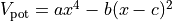 where
where  is the position
and
is the position
and  ,
,  and
and  are potential parameters.
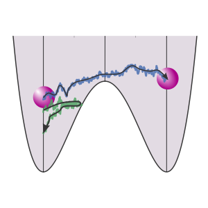
Fig. 8 Illustration of the potential energy and two trajectories: one is reactive (giving a transition), while the other is non-reactive.
The script for running a RETIS simulation can be downloaded here:
retis_movie.py.
But before we can run this script, we need to install the PyRETIS library and
matplotlib:
The PyRETIS library is distributed in the Python Package Index and can be installed using pip:[1]
pip install pyretis
If you want to install the library system-wide, you will need super-user access (typically a sudo will do). If you don’t have super-user access, pip works well with virtualenv and we refer to the virtualenv user guide for more information about setting this up. [2]
Note: If you have a previous installation of PyRETIS (the newest release is version 3.0.0), it can be upgraded using
pip install --upgrade pyretis
Matplotlib can also be installed using pip. However, for the best performance we recommend that you follow a guide specific for your operative system. Please see the matplotlib documentation. [3] If you are sure that all matplotlib requirements are satisfied, you can install it directly using pip:
pip install matplotlib
After installing the PyRETIS library, please check that is has been properly set up by running the following command (at the command line):
python -c 'import pyretis; print(pyretis.__version__)'
which should print out the version of your installed PyRETIS library.
Running the example script
Download the example script retis_movie.py
to a location on your computer. Now this script can be executed by running
python retis_movie.py
which should display an animation similar to the image shown below.
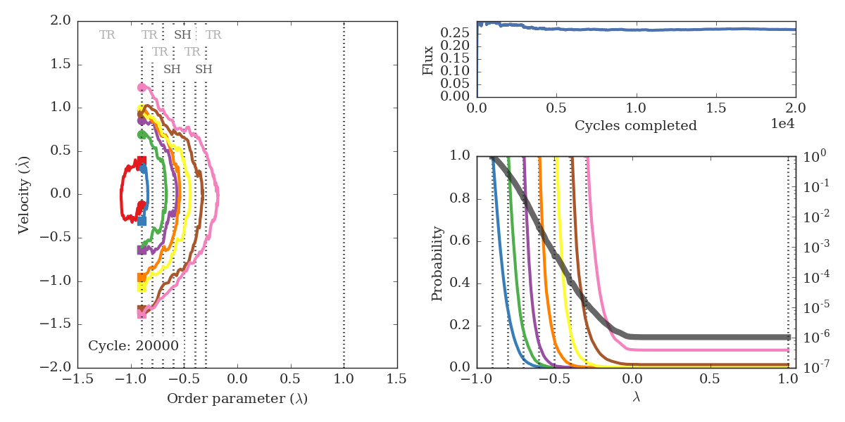
Fig. 9 Snapshot from the RETIS animation. The left panel shows accepted trajectories for the different ensembles and the upper text shows the kind of move performed: TR = Time Reversal, SH = Shooting, NU = Null (no move) and SW = Swapping. The upper right panel displays the calculated initial flux, while the lower right panel shows the probabilities for the different ensembles (values on the left y-axis) and the overall matched probability (in gray, values on the right y-axis). Vertical dotted lines display the positions of the RETIS interfaces.
The bulk of this script handles the plotting, and we will not go into details on how matplotlib is used to plot the result. We will in the following show highlight some changes you can do to modify the RETIS simulation.
If you complete the full 20000 cycles, you can compare your results with the previously reported data of van Erp. [4] [5]
Modifying the RETIS simulation
The dictionary SETTINGS in the retis_movie.py script defines
the simulation. Changing the values in this dictionary will modify the simulation.
Here are some examples:
Changing the number of steps:
The number of steps is changed by changing the dictionary for
SETTINGS['simulation']. From 20000 stepsSETTINGS['simulation'] = {'task': 'retis', 'steps': 20000}
to just 100:
SETTINGS['simulation'] = {'task': 'retis',
                          'steps': 100}
Changing the interfaces:
The interfaces are defined in a list:
SETTINGS['interfaces'] = [-0.9, -0.8, -0.7, -0.6, -0.5, -0.4, -0.3, 1.0]
We can, for instance, see what happens if we just use two interfaces:
SETTINGS['interfaces'] = [-0.9, 1.0]
Changing the temperature:
The temperature is defined by:
SETTINGS['system'] = {'units': 'lj', 'temperature': 0.07}
and can be changed by giving it a different value:
SETTINGS['system'] = {'units': 'lj', 'temperature': 0.21}
Changing the potential parameters:
The potential parameters is defined by:
SETTINGS['potential'] = [{'a': 1.0, 'b': 2.0, 'c': 0.0,
                          'class': 'DoubleWell'}]
We can change the parameters directly, e.g.:
SETTINGS['potential'] = [{'a': 0.5, 'b': 1.0, 'c': 0.0,
                          'class': 'DoubleWell'}]
Note: It is a good idea to plot the potential if you change the parameters. This will allow you to check the position of the interfaces.
References
| [1] | The pip user documentation, https://pip.pypa.io/en/stable |
| [2] | The virtualenv user guide, https://virtualenv.pypa.io/en/stable/userguide/ |
| [3] | The matplotlib installation instructions, http://matplotlib.org/users/installing.html |
| [4] | Titus S. Van Erp, Dynamical Rare Event Simulation Techniques for Equilibrium and Nonequilibrium Systems, Advances in Chemical Physics, 151, pp. 27 - 60, 2012, http://dx.doi.org/10.1002/9781118309513.ch2 |
| [5] | https://arxiv.org/abs/1101.0927 |