Molecular modelling: Introduction to RETIS¶

Table of Contents

Introduction
Installing PyRETIS and running the exercise
- Installing PyRETIS
- Running the exercise
Part 1 - Introduction
Part 2 - Improving the efficiency
References

Introduction ¶

In this exercise, you will explore a rare event with the Replica Exchange Transition Interface Sampling (RETIS) algorithm.

We will consider a simple 1D potential where a particle is moving. The potential is given by $V_{\text{pot}} = x^4 - 2 \times x^2$ where $x$ is the position. By plotting this potential, we see that we have two states (at $x=-1$ and $x=1$ ) separated by a barrier (at $x=0$ ):

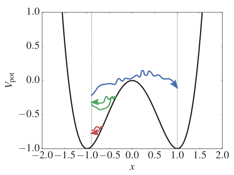
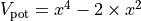
Fig. 5 The potential energy as a function of the position. We have two stable states (at x = -1 and x = 1) separated by a barrier (at x = 0). In addition, three paths are shown. One is reactive while the two others are not able to escape the state at x = -1. Using the RETIS method, we can generate such paths which gives information about the reaction rate and the mechanism. The vertical dotted lines show two RETIS interfaces.¶

Using the RETIS algorithm, we will compute the rate constant for the transition between the two states. We will also try to position the RETIS interfaces to maximise the efficiency of our calculation. The exercise is structured as follows:

Installing PyRETIS and running the exercise. Short version:
- Install PyRETIS (pip install pyretis)
- Install matplotlib (pip install matplotlib)
- Download retis.py
- Download retis_movie.py
Part 1 - Introduction
Part 2 - Improving the efficiency
References

How to pass:

From Part 2 - Improving the efficiency, show the teaching assistant the results from your best simulation. Here, “best” is the simulation with the fewest force evaluations and lowest uncertainties for a fixed number of steps as specified in the exercise. The results to show the teaching assistant are the interfaces you have used, the number of force evaluations, the initial flux, the crossing probability and rate constant with error estimates.

Installing PyRETIS and running the exercise ¶

Installing PyRETIS ¶

In this example, we will make use of the PyRETIS library for carrying out the RETIS simulations and we will use matplotlib for plotting some results. These two libraries will have to be installed before we start:

The PyRETIS library is distributed in the Python Package Index and can be installed using pip. [1] Typically, pip is included when you install Python, but if this is not the case you can install it manually. This can be done by following the installation pip installation instructions:
1. Download the get-pip.py script from the pip web-page.
2. Install pip using the terminal:
```
python get-pip.py
```
  or
```
python get-pip.py --user
```
  The --user option will allow you to install pip locally for your own user when you do not have super-user access to the computer you are working on.
As already mentioned, the PyRETIS library is distributed in the Python Package Index and can be installed using pip [1] and the following command:
```
pip install pyretis
```
Note that this command might require you to have super-user access. If this is not the case, you can try to install PyRETIS locally for your own user using a virtual environment or with pip locally:
```
pip install pyretis --user
```
For information about setting up a virtual environment, we refer to the virtualenv user guide. [2]

Note: If you have a previous installation of PyRETIS (the newest released version is: 3.0.0), it can be upgraded using
```
pip install --upgrade pyretis
```
Matplotlib can also be installed using pip. However, for the best performance we recommend that you follow a guide specific for your operative system. Please see the matplotlib documentation. [3] If you are sure that all matplotlib requirements are satisfied, you can install it directly using pip:
```
pip install matplotlib
```

Running the exercise ¶

We will use two Python scripts in this example to run the RETIS simulation. One will display an animation on the fly, while the other script will just output some text results.

Download the example script retis_movie.py to a location on your computer. This script can be executed by running the command

python retis_movie.py

in your terminal. This should display an animation similar to the image shown below.

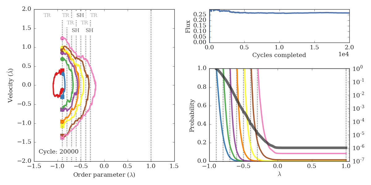
Fig. 6 Snapshot from the RETIS animation. The left panel shows accepted trajectories for the different ensembles and the upper text shows the kind of move performed: TR = Time Reversal, SH = Shooting, NU = Null (no move) and SW = Swapping. The upper right panel displays the calculated initial flux, while the lower right panel shows the probabilities for the different ensembles (values on the left y-axis) and the overall matched probability (in gray, values on the right y-axis). Vertical dotted lines display the positions of the RETIS interfaces.¶

The bulk of this script handles the plotting, and we will not go into details on how matplotlib is used to plot the result. We will rather focus on the RETIS algorithm and how we can use it to calculate rate constants. But before we do that, let us also try the text-based script. This script will give the same output as the retis_movie.py script, but it will not display the animation and will thus run slightly faster. Download the example script retis.py to a location on your computer and execute it by running the command

python retis.py > name_of_file.txt

which should display a progress bar showing estimating the time left for your simulation. In addition, text output from the simulation is written to the file name_of_file.txt:

Fig. 7 Sample output from the text-based RETIS script. The top terminal is running the simulation where the progress meter is displayed. The lower terminal is inspecting the output file. After each completed RETIS cycle the script outputs the cycle number, and then some results for each ensemble. The ensemble names are given in the first column, the type of move executed is shown in the next column, the status after the move and the current estimate of the crossing probability ( $P_\mathrm{cross}$ ) for each ensemble in the two following columns. Then the current estimates for the flux, the crossing probability and the rate constant is outputted. Finally, the number of force evaluations are given.¶

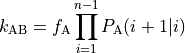
The RETIS method which is used in this exercise aim to calculate the rate constant $k_{\text{AB}}$ for the transition between the two states shown in Fig. 5. This is accomplished by generating reactive trajectories connecting the reactant state and the product state. We define these two states using two interfaces (the vertical lines in Fig. 5) which we label $\lambda_\text{A}$ and $\lambda_\text{B}$ respectively. That is, left of $\lambda_\text{A}$ corresponds to the reactant state and right of $\lambda_\text{B}$ corresponds to the product state. Since the probability for the actual crossing can be very small, we introduce several more interfaces which help us obtain the crossing probability. These interfaces define the so-called path ensembles, labeled $[0^-], [0^+], [1^+], \ldots$ and so on as shown in Fig. 7. The path ensemble $[i^+]$ contain trajectories that start at $\lambda_\text{A}$ , then cross an intermediate interface $\lambda_i$ before reaching $\lambda_\text{B}$ or returning to $\lambda_\text{A}$ . As you may have noticed, there is a special path ensemble labelled $[0^-]$ which contains paths that start at $\lambda_\text{A}$ , then go in the opposite direction (i.e. to the left of $\lambda_\text{A}$ ) before returning to $\lambda_\text{A}$ . This ensemble is used to calculate how often we cross $\lambda_\text{A}$ and head towards the product state at $\lambda_\text{B}$ . Now, if we know how often we cross $\lambda_\text{A}$ and head for the product state and the probability of reaching this state given that we crossed $\lambda_\text{A}$ then the rate constant can be obtained according to

$k_{\text{AB}} = f_{\text{A}} \prod_{i=1}^{n-1} P_{\text{A}} (i+1|i)$

where $f_{\text{A}}$ is the initial flux and $P_{\text{A}} (i+1|i)$ are intermediate crossing probabilities, obtained using the different path ensembles. The initial flux is obtained using the path lengths in ensembles $[0^-]$ and $[0^+]$ as

$f_{\text{A}} = (\langle t_{\text{path}}^{[0^-]} \rangle + \langle t_{\text{path}}^{[0^+]} \rangle)^{-1}$

where $\langle t_{\text{path}}^{[k]} \rangle$ denotes the average path length in ensemble $[k]$ . The intermediate probability $P_{\text{A}} (i+1|i)$ is the probability of path reaching the next ( $i+1$ ) interface given that it originated in $\lambda_\text{A}$ , ended in $\lambda_\text{A}$ or $\lambda_\text{B}$ and had at least one crossing with $\lambda_\text{i}$ . This probability can be obtained as the fraction of paths in the $[i^+]$ ensemble that cross $\lambda_{i+1}$ . It is these probabilities that are labelled $P_\text{cross}$ in Fig. 7.

The optimal number of path ensembles to use in a RETIS simulation is a trade-off between not having to do too many path simulations and not having too small crossing probabilities (the $P_\text{cross}$ -values in Fig. 7). By making some basic assumptions on the path lengths etc. one can establish a theoretical optimum which should be obtained when all crossing probabilities are around 0.2 (the derivation of this can be found in Ref. [6]). However, the assumptions are never completely valid in realistic systems. Hence, the optimum is presumably close to having all probabilities equal to 0.2 but not exactly (but somewhere in the range 0.1 till 0.9).

As stated above, the RETIS method generate reactive trajectories connecting the initial and final state using the moves shown in Fig. 7 and described in Table 45. The outcome of each attempted RETIS move is given a three letter abbreviation as described in Table 46.

Table 45 Abbreviations for the RETIS moves¶
Abbreviation	Description
`swap`	A RETIS swapping move.
`nullmove`	Just accepting the last accepted path once again.
`tis (sh)`	A TIS shooting move
`tis (tr)`	A TIS time-reversal move

Table 46 Abbreviations for the RETIS statuses¶
Abbreviation	Description
`ACC`	The path has been accepted.
`BWI`	When integrating backward in time for a shooting move we arrived at the right interface and not the left one, i.e. we reached the Wrong Interface.
`BTL`	When integrating backward in time for a shooting move, the backward trajectory will have a maximum length determined by the RETIS algorithm in order to obey detailed balance. This maximum varies each time: it is the old path length divided by a random number between 0 and 1. `BTL` means that we did not reach any of the outer most interfaces before we exceeded this maximum path length.
`BTX`	We also have a maximum length for trajectories in order to limit the memory the trajectories use. `BTX` means that the trajectory length exceeded this limit before we reached an interface. This limit implies that we ignore very long trajectories and, therefore, it will result in a systematic error. The number of `BTX` or `FTX` occurrences can be reduced by increasing the parameter `maxlength` in the input script.
`FTL`	Similar to `BTL` in the Forward direction.
`FTX`	Similar to `BTX` in the Forward direction.
`NCR`	No crossing with the interface which has to be crossed in order to be part of the specific path ensemble. This can happen when we attempt swapping move or when the shooting move goes backward and forward in time to the left interface without making sufficient progress along the reaction coordinate.

Now, hopefully, you are able to execute the two example scripts we will be using.

Before we start with the exercise we give a few examples on how you can change the input scripts in order to modify your simulation. Typically, this involves making changes in the SETTINGS dictionary defined in the Python scripts. In fact the RETIS simulation you are running is defined with this Python dictionary. In this exercise, we will just change a few of these settings and we give some examples here:

In order to run a longer simulation you need to change the steps keyword. For instance from 150 steps to 20000. If you run the simulation for 20000 steps you can compare your results with the previously reported data of van Erp. [4] [5] The required change is from:

SETTINGS['simulation'] = {'task': 'retis',
                          'steps': 150,
                          'interfaces': INTERFACES}

to:

SETTINGS['simulation'] = {'task': 'retis',
                          'steps': 20000,
                          'interfaces': INTERFACES}

The number of interfaces to use in the RETIS algorithm is defined in a list:
```
INTERFACES = [-0.9, -0.8, -0.7, -0.6, -0.5, -0.4, -0.3, 1.0]
```
We can, for instance, see what happens if we just use fewer interfaces:
```
INTERFACES = [-0.9, -0.8, -0.6, -0.4, -0.3, 1.0]
```
We can also change settings for the RETIS algorithm itself:

The settings for the RETIS method is split into two parts, one is RETIS specific and the other is TIS specific. The former controls swapping while the latter the shooting. In this exercise, we will just change the frequencies of the different moves. The percentage of swapping are controlled by the swapfreq keyword of the RETIS settings:
```
# RETIS specific settings:
SETTINGS['retis'] = {'swapfreq': 0.5,
                     'nullmoves': True,
                     'swapsimul': True}
```
Here, 50 % (a fraction of 0.5) will be swapping moves. What about the remaining 50% of the moves? These will be TIS moves and here we have two options - shooting or time reversal. The relative frequency of these moves is determined by the freq keyword in the TIS specific settings.
```
# TIS specific settings:
SETTINGS['tis'] = {'freq': 0.5,
                   'maxlength': 20000,
                   'aimless': True,
                   'allowmaxlength': False,
                   'sigma_v': -1,
                   'seed': 0,
                   'zero_momentum': False,
                   'rescale_energy': False}
```
Here, 50% will be shooting moves and 50% will be time-reversal moves. Note that this is as a percentage of the TIS moves, so in total, we will have 50% swapping, 25% shooting and 25% time reversal.

What happens with a swapfreq equal to 0.8 and a freq equal to 0.6? We will have 80% swapping moves, 12% ( $0.2\times0.6$ ) time reversal moves and 8% ( $0.2 \times (1-0.6)$ ) shooting moves.

Part 1 - Introduction ¶

We will warm up with a few questions about the RETIS method and we will run a few short simulations to see how the method works in practice.

What “problem” are we solving with the RETIS method? Why don’t we just run a brute-force simulation?
How would you (in just a few sentences) describe what happens when you run a RETIS simulation. Some keywords to get you started: swapping, shooting, time-reversal, path ensembles, rate, crossing probability… Here you can also try to explain what is displayed in the animation shown by running retis_movie.py.
In the RETIS method, we have three main moves which generate new paths. These are the shooting, time-reversal and swapping moves. How do these moves generate new paths? Which move is the most computationally demanding? Which one is the least computationally demanding?
Let us check your answers to the previous question by performing two short RETIS simulations with the retis_movie.py script using different swapping frequencies. One of the outputs from the retis_movie.py script is the number of force evaluations which is a measure of the computational cost. Compare the total number of force evaluations in these two cases:
1. Set steps to 1000 and swapfreq to 0.2 and run a RETIS simulation using:
```
python retis_movie.py > swap-0.2.txt
```
2. Set steps to 1000 and swapfreq to 0.8 and run a RETIS simulation using:
```
python retis_movie.py > swap-0.8.txt
```
In which of these two cases are the number of force evaluations greatest? Does this agree with your answer to question 3? What happens if you increase the freq keyword? Is this as expected? Note that the total number of force evaluations can be found at the end of the text output from the script.
Why do we use so many path ensembles in our RETIS simulation? Explore what happens when you change the number of interfaces in the retis_movie.py script. For instance, reduce the number of interfaces to just two:
```
INTERFACES = [-0.9, 1.0]
```
and set the number of steps to 4000. Do you expect this to change the total number of force evaluations dramatically, compared to a case with 8 interfaces running for 1000 steps? Compare with a simulation using the interfaces
```
INTERFACES = [-0.9, -0.8, -0.7, -0.6, -0.5, -0.4, -0.3, 1.0]
```
for 1000 steps. In these two simulations you can also set
```
PCROSS_LOG = True
```
to show the crossing probabilities on a log scale.
The swapping move is the defining move for the RETIS algorithm and is essentially the move that separates it from the TIS algorithm. What is the purpose of the swapping move? What will happen if we remove it? Investigate this using the retis_movie.py script and setting the frequency of swapping moves to 0. Here, you can run 1000 steps and compare with the output from the previous question. Use the same 8 interfaces and set PCROSS_LOG = TRUE.

Part 2 - Improving the efficiency ¶

In the last part in the previous section, you ran several very short RETIS simulation. Here we will run some longer simulations and we will see how efficiently we can run the RETIS simulations. For instance, if we set the interfaces to

INTERFACES = [-0.9, -0.8, -0.7, -0.6, -0.5, -0.4, -0.3, 1.0]

steps to 2000 and the frequencies to 0.5, the output will be similar to:

# Flux: 0.285125 +- 0.00956114
# Crossing probability: 8.10682e-07 +-4.9152e-07
# K_AB: 2.31146e-07 +- 1.40359e-07

with a total number of force evaluations equal to about 3.9 million. As you can see there are rather large uncertainties, because 2000 is in fact a small number of steps. In this part of the exercise, we will see if we can improve the situation and our goal is to lower (if possible) the number of force evaluations and the uncertainty. Here, you can proceed as you like, but to get you started here are some suggestions:

First, consider how you would compare two simulations. Say that we have the following results:
1. A simulation with $10^6$ force evaluations and an error (relative) in the rate constant of 10%.
2. A simulation with $2\times 10^6$ force evaluations and an error (relative) in the rate constant of 5%.
Which one of these two simulations would you say performs better?
Run first some short simulations (say 100-200 steps) where you test out different positions of interfaces and also a different number of interfaces. Here you should make use of both the retis_movie.py and retis.py scripts to investigate how your changes influence the results.
After having found a set of interfaces you are happy with, run a longer simulation (2000 steps) with the retis.py script and report your results to the teaching assistant. How do your results compare to the results given above? Are you able to perform better? Note: It will take around 7-8 minutes to complete the 2000 cycles.

References ¶

[1]	(1, 2) The pip user documentation, https://pip.pypa.io/en/stable

[2]	The virtualenv user guide, https://virtualenv.pypa.io/en/stable/userguide/

[3]	The matplotlib installation instructions, http://matplotlib.org/users/installing.html

[4]	Titus S. Van Erp, Dynamical Rare Event Simulation Techniques for Equilibrium and Nonequilibrium Systems, Advances in Chemical Physics, 151, pp. 27 - 60, 2012, http://dx.doi.org/10.1002/9781118309513.ch2

[5]	https://arxiv.org/abs/1101.0927

[6]	http://dx.doi.org/10.1016/j.jcp.2004.11.003

Molecular modelling: Introduction to RETIS¶

Introduction¶

Installing PyRETIS and running the exercise¶

Installing PyRETIS¶

Running the exercise¶

Part 1 - Introduction¶

Part 2 - Improving the efficiency¶

References¶